4.1.1 Pre-analysis Data Exploration
Since the outcome variable is delay time, a continuous variable, we
want to fit a linear regression model. However, the scale of outcome
data (from 0 to +∞) is a problem since it does not in consistent with
the scale of linear function (from -∞ to +∞). To make them in agreement,
we decided to normalize the outcome data with log transformation and
scale it to -∞ to +∞. At the meanwhile, this log transformation also
solved the terrible skewness observed in the distribution of delay time.
After this step, our outcome variable change from delay time to log
(delay time), in which still representing the delay time.
NOTE: We do have plenty of outliers with
extreme long delay time, however, considering these extreme observations
could be indicative to the underlying relationship, we chose not to
exclude them. After log transformation, the outlier issues were no
longer too scary.
What we did next is to check if there are any associations existing
between the independent variables and the dependent variable (i.e., log
(delay time)).
By plotting boxplots, doing ANOVA and pairwise comparisons for
groups of our categorical independent variables, we found all 3
variables are highly significantly associated with the outcome, with
p-value (< 2e-16), and thus we decided to include these 3 categorical
variables (i.e., airlines, months,
time of the day) into the final model.
By plotting scatterplots, calculating Pearson correlation
coefficients for all continuous variables, we did not find any
significant linear association between independent variables and delay
time. However, considering the fact that we do not have perfect data
source and limited data collection interval, which all might bias the
scatterplot as well as the correlation, we identified 2 variables with
correlation coefficients greater than 0.3 (moderate correlation) and we
decided to include these 2 continuous variables (i.e.,
carrier delay time and
late arrival delay time) into the model for prediction
purpose.
4.1.2 Model Fitting
From the previous data exploration and visualization, we found some
interesting trends that we all think worthy further inspection and can
be the potential independent variables for the prediction of delay in
time.
Given the above information, we came up 2 rationales for building the
linear regression model:
- Based on observed relationship only:
Include the 5 variables we identified above.
Model 1: delay ~ airline + month + time of the day + carrier delay
time + late arrival delay time
|
r.squared
|
statistic
|
p.value
|
df
|
|
0.4220695
|
602.9567
|
<2.2e-16
|
13
|
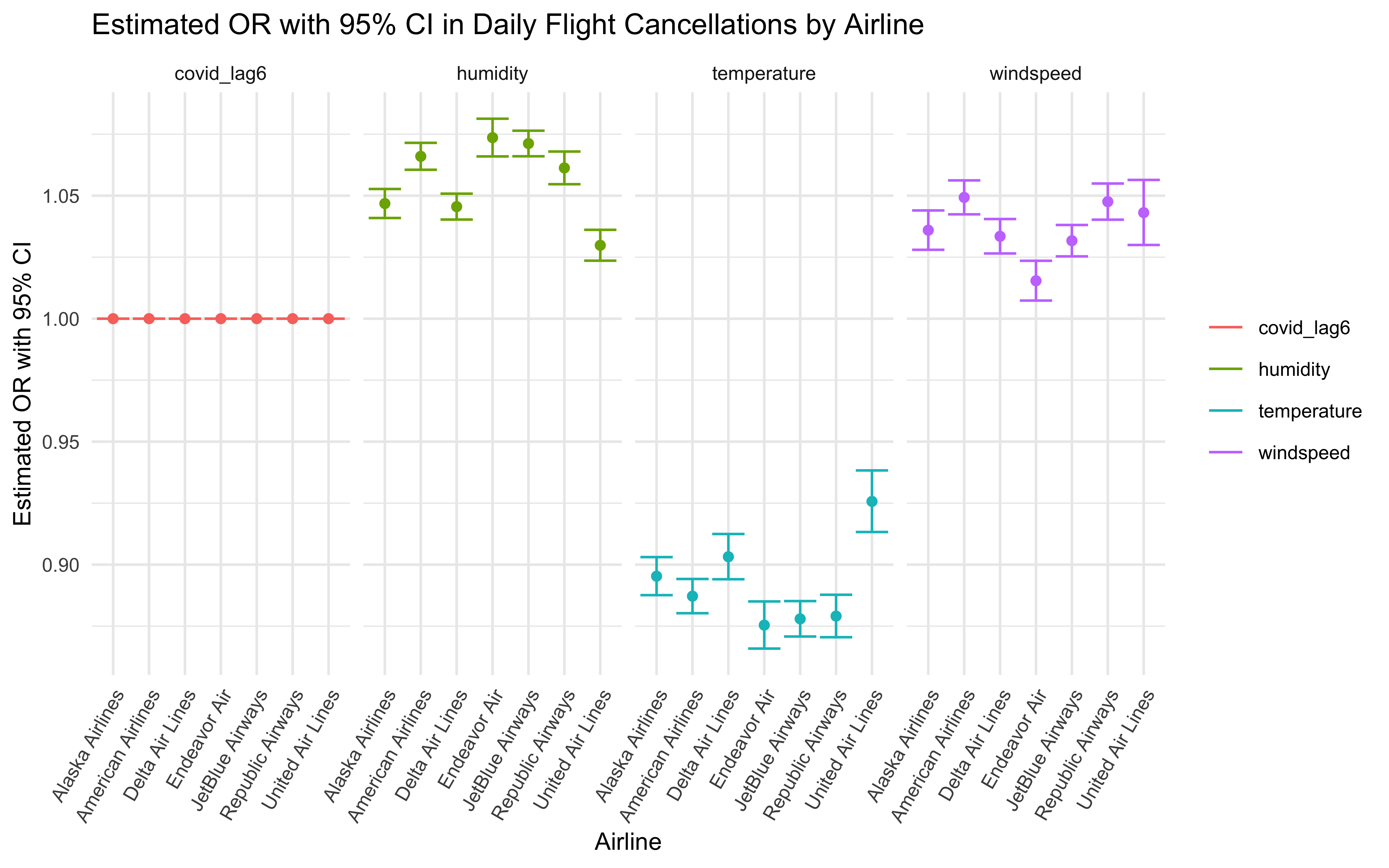
- Based on both common sense and observed relationship:
Except for the 5 variables identified above, we also hypothesize
the rest of variables (i.e., extreme weather delay time, NAS delay time,
security delay time, temperature, humidity, visibility, wind speed)
would affect the delay time based on our common sense and
experience.
Model 2: delay ~ airline + month + time of the day + carrier delay
time + late arrival delay time + extreme weather delay time + NAS delay
time + security delay time + temperature + humidity + visibility + wind
speed
|
r.squared
|
statistic
|
p.value
|
df
|
|
0.4524891
|
443.2239
|
<2.2e-16
|
20
|
Besides, from previous data exploration focusing on interactions
between independent variables, we identified 3 interaction terms (i.e.,
Temperature * Month, Carrier * Airline,
Month * Airline) that have the potential to be added into
the final model.
So, next we did cross validation to figure out the best model.
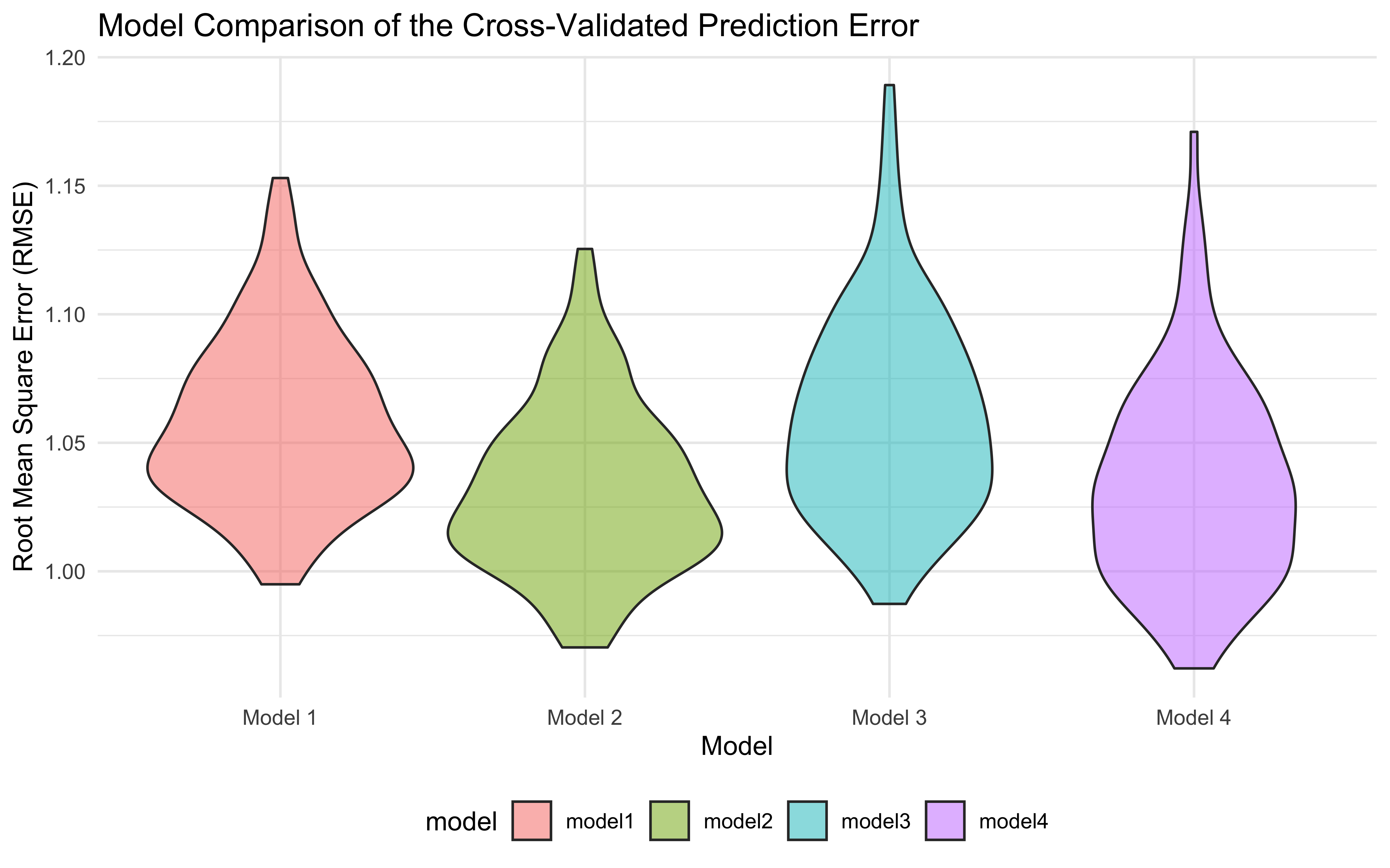
It turns out that Model 1 is the best model, with similar RMSE value
with the other three but fewest number of model parameters. For
parsimony purpose, we chose Model 1 as the final model.
4.1.2 Model Diagnostics
The last step about building predictive model will be the model
diagnostics, where we plot residuals against fitted value to see if our
model has a good fit and prediction power.
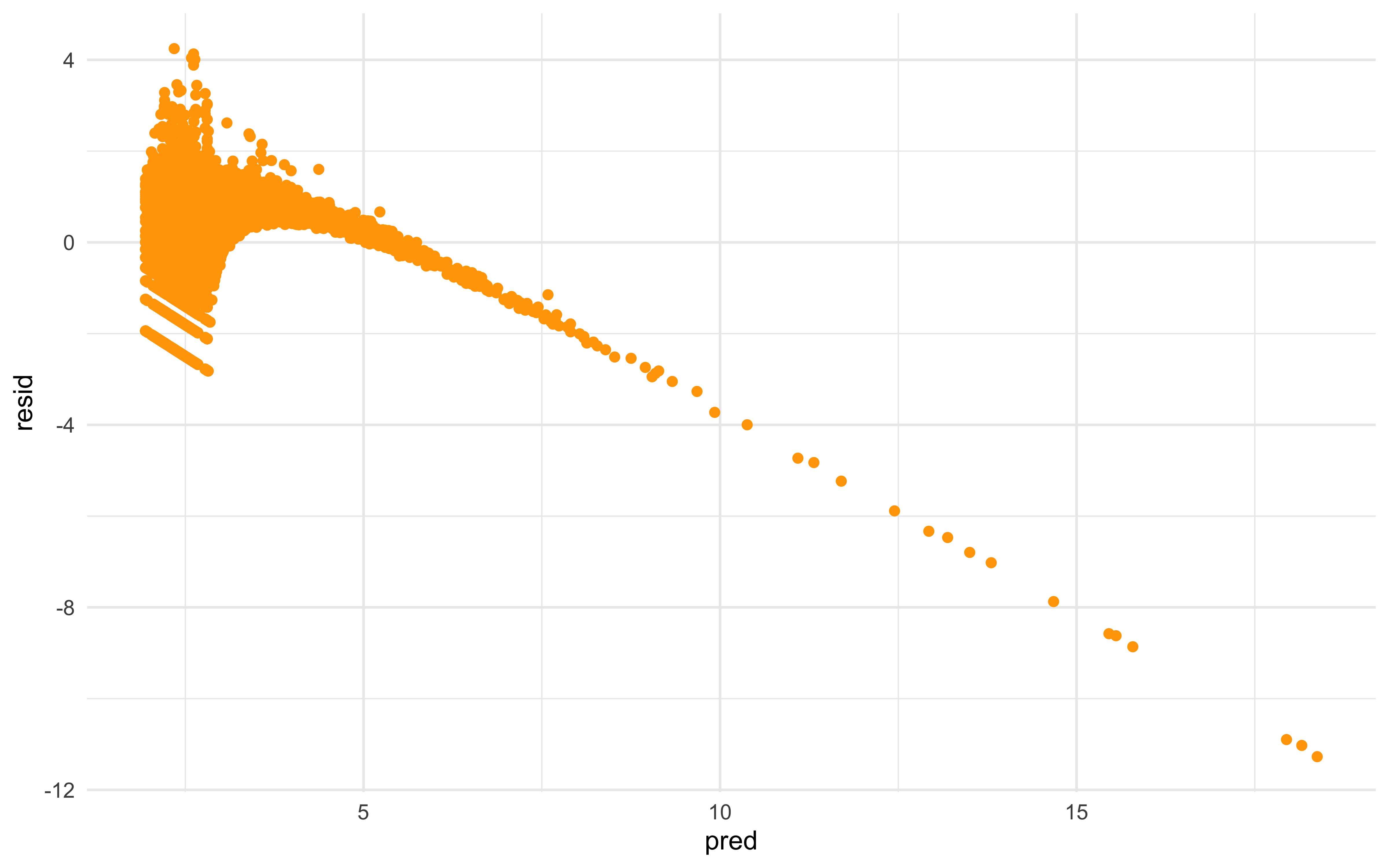
Unfortunately, the answer is NO.